Inferential Statistics

I.DISTRIBUTIONS

Definition:
- In statistics, when we talk about distributions we usually mean probability distributions.
- Definition (informal): a distribution is a function that shows the possible values for a variable and how often they occur.
- Definition (Wikipedia): In probability theory and statistics. a probability distribution is a mathematical function that, stated in simple terms, can be thought of as providing the probabilities of occurrence possible outcomes in an experiment.
- Example: Normal distribution, Student's T distribution, Poisson distribution, Uniform distribution, Binomial distribution.
Graphical representation:
- It is a common mistake to believe that the distribution is the graph. In fact the distribution is the 'rule' that determines how values are positioned in relation to each other.
- Very often, we use a graph to visualize the data. Since different distributions have a particular graphical representation, statisticians like to graph them.

Type	Graph
Uniform Distribuiton
Binomial Distribution
Normal Distribution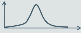
Student's T distribution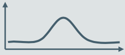

II.THE NORMAL DISTRIBUTION:

The normal distribution is also known as Gaussian distribution or the Bell curve. It is one of the most common distributions due to the following reasons:
- It approximates a wide variety of random variables
- Distributions of sample means with large enough samples sizes could be approximated to normal
- All computable statistics are elegant
- Heavily used in regression analysis
- Good track record
Examples:
- Biology. Most biological measures are normally distributed, such asL height, length of arms, legs, nails, blood pressure; thickness of tree barks, etc.
- IQ tests
- Stock market information

Normal Distribution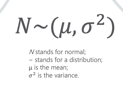
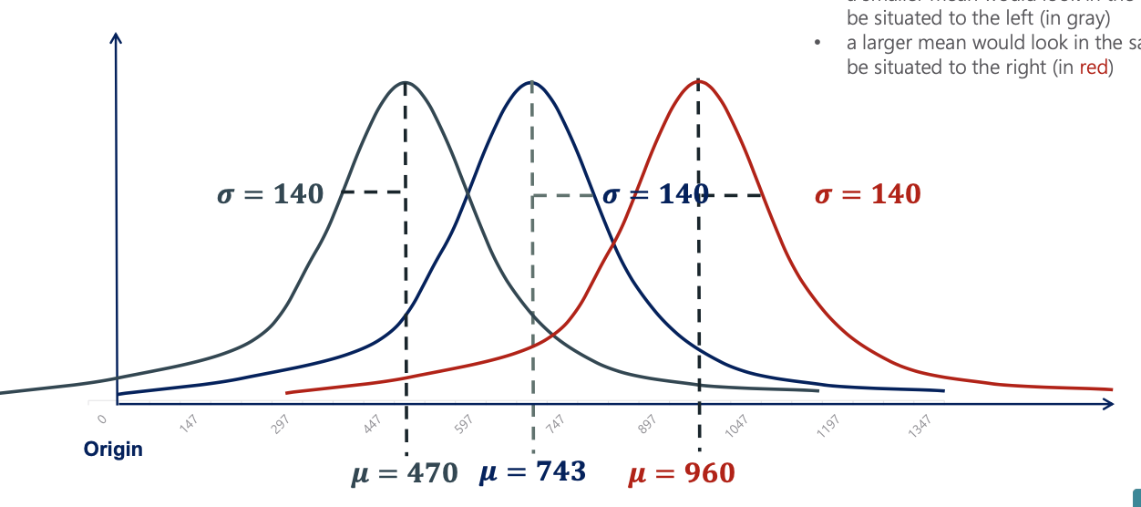
Keeping the standard deviation constant, the graph of a normal distribution with: - a smaller mean would look in the same way, but be situated in the left (gray) - a larger mean would look in the same way, but be situated to the right (red)
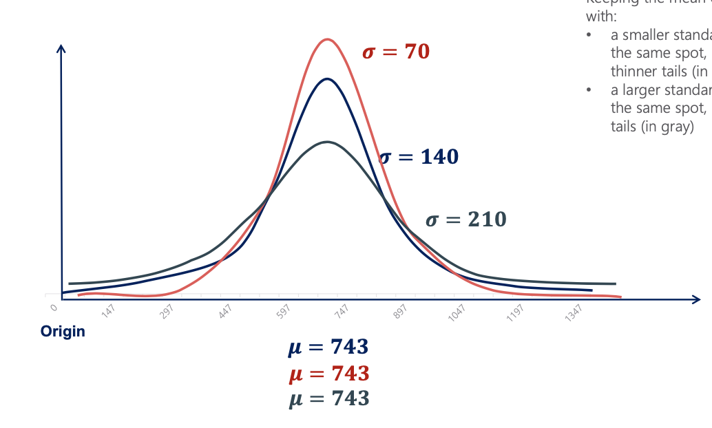
Keeping the mean constant, a normal distribution with: - a smaller standard deviation would be situated in the same spot, but have a higher peak and thinner tails (red) - a larger standard deviation would be situated in the same spot, but have a lower peak and fatter tails (gray) - The lower the standard deviation, the more accurate, or the higher confidence level.

III.THE STANDARD NORMAL DISTRIBUTION:

The Standard Normal distribution is a particular case of the Normal distribution. It has a mean of 0 and a standard deviation of 1.
Every Normal distribution can be 'standardized' using the standardization formula:
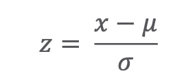
A variable following the Standard Normal distribution is denoted with the letter z.
Why standardize?
Standardization allows us to:
- Compare different normally distributed datasets
- detect normality
- detect outliers
- create confidence intervals
- test hypotheses
- perform regression analysis
- Denote: N~(0,1)
- Rationale of the formula for standardization:
  We want to transform a random variable from . Subtracting the mean from all observations would cause a transformation from , moving the graph to the origin. Subsequently, dividing all observations by the standard deviation would cause a transformation from , standardizing the peak and the tails of the graph.
  IV.THE CENTRAL LIMIT THEOREM:
The Central Limit Theorem (CLT) is one of the greatest statistical insights. It states that no matter the underlying distribution of the dataset, the sampling distribution of the means would approximate a normal distribution. Moreover, the mean of the sampling distribution would be equal to the mean of the original distribution and the variance would be n times smaller, where n is the size of the samples. The CLT applies whenever we have a sum or an average of many variables (e.g sum of rolled numbers and rolling dice)
Why is it useful?: The CLT allows us to assume normality for many different variables. That is very useful for confidence intervals, hypothesis testing, and regression analysis. In fact, the Normal distribution is so predominantly observed around us due to the fact that following the CLT, many variables converge to Normal.
- Where can we see it?: Since many concepts and events are a sum or an average of different effects, CLT applies and we observe normality all the time. For example, in regression analysis, the dependent variable is explained through the sum of error terms.
  V.ESTIMATORS AND ESTIMATES:

ESTIMATORS	ESTIMATES
- Broadly, an estimator is a mathematical function that approximates a population parameter depending only on sample information. - Examples of estimators and the corresponding parameters: - Estimators have two important properties: - Bias: the expected value of an unbiased estimator is the population parameter. The bias in this case is 0. If the expected value of an estimator is (parameter + b), then the bias is b. - Efficiency: the most efficient estimator is the one with the smallest variance.	- An estimate is the output that you get from the estimator (when you apply the formula). There are two types of estimates: point estimates and confidence interval estimates. - Point estimates: - A single value - E.g: 1, 5, 122.7, 0.32 - Confidence intervals: - An interval. - E.g: (1, 5); (12, 23); (-0.71, 0.11) - Confidence intervals are much more precise than point estimates. That is why they are prefered when making inferences

ESTIMATORS

ESTIMATES

- Broadly, an estimator is a mathematical function that approximates a population parameter depending only on sample information.
- Examples of estimators and the corresponding parameters: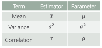

- Estimators have two important properties:
- Bias: the expected value of an unbiased estimator is the population parameter. The bias in this case is 0. If the expected value of an estimator is (parameter + b), then the bias is b.
- Efficiency: the most efficient estimator is the one with the smallest variance.

- An estimate is the output that you get from the estimator (when you apply the formula). There are two types of estimates: point estimates and confidence interval estimates.
- Point estimates:
- A single value
- E.g: 1, 5, 122.7, 0.32
- Confidence intervals:
- An interval.
- E.g: (1, 5); (12, 23); (-0.71, 0.11)
- Confidence intervals are much more precise than point estimates. That is why they are prefered when making inferences

VI.CONFIDENCE INTERVALS AND THE MARGIN OF ERROR:

Definition: a confidence interval is an interval within which we are confident (with a certain percentage of confidence) the population parameter will fall. We build the confidence interval around the point estimate.
You can never be 100% confident unless you went through all of the population.
- (1 - a) is the level of confidence. We are (1 - a)*100% confident that the population parameter will fall in the specified interval. Common alphas are 0.01, 0.05, 0.1
- VII.STUDENT'S T DISTRIBUTION:
The student's T distribution is used predominantly for creating confidence intervals and testing hypotheses with normally distributed populations when the sample sizes are small. It is particularly useful when we don't have enough information or it is too costly to obtain it.
All else equal, the Student's T distribution has fatter tails than the Normal distribution and a lower peak. This is to reflect he higher level of uncertainty, cause by the small sample size.
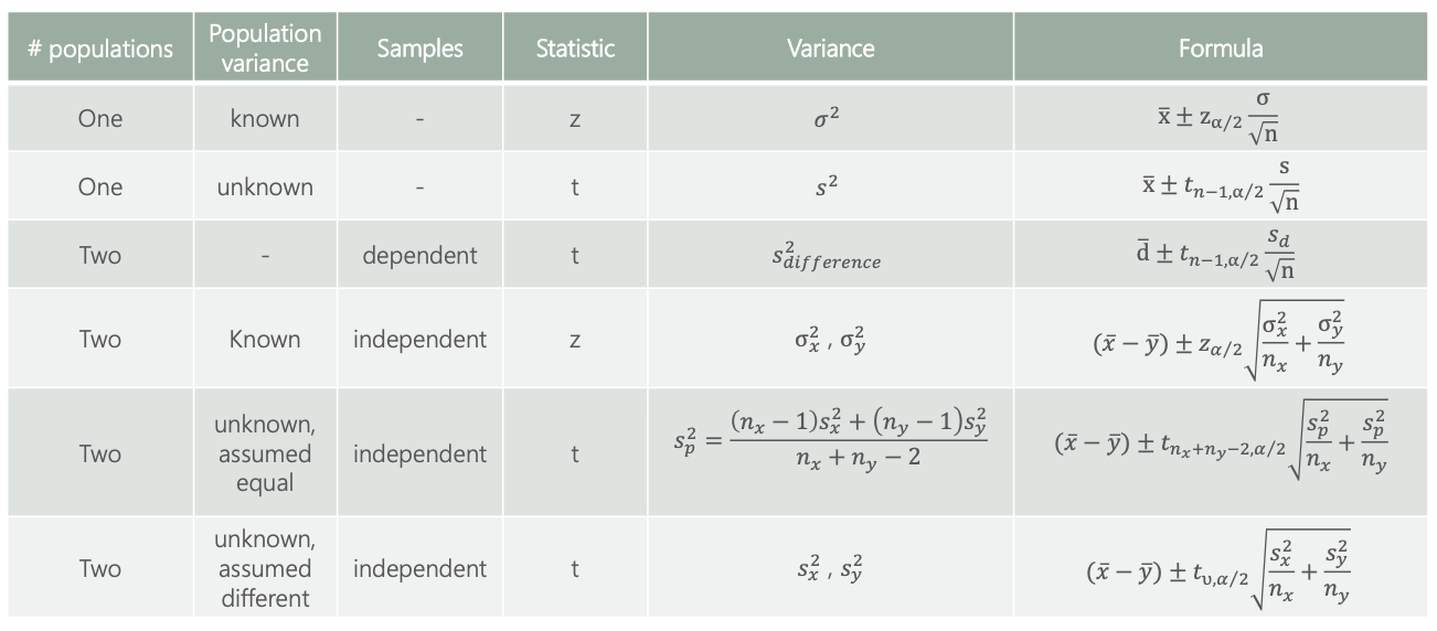
VIII.FORMULAS FOR CONFIDENCE INTERVALS